Last Update: 17 September 2023
Download RMarkdown:
GRWG_Maps.Rmd
Overview
This tutorial covers creating maps in R using the sf and ggplot2
packages.
To download the Rmarkdown file for this tutorial to your local machine (or any SCINet cluster within OoD), you can use the following lines:
library(httr)
tutorial_name <- 'GRWG_Maps.Rmd'
GET(paste0('https://geospatial.101workbook.org/tutorials/',tutorial_name),
    write_disk(tutorial_name))
Language: R
Primary Libraries/Packages:
| Name | Description | Link |
|---|---|---|
| sf | Simple Features for R | https://r-spatial.github.io/sf/ |
| ggplot2 | Create Elegant Data Visualizations Using the Grammar of Graphics | https://ggplot2.tidyverse.org/ |
Nomenclature
- Raster: Data defined on a grid of geospatial coordinates
- CRS: Coordinate Reference System, also known as a spatial reference system. A system for defining geospatial coordinates.
Data Details
- Data: FS National Forests Dataset (US Forest Service Proclaimed Forests)
- Link: https://www.geoplatform.gov/metadata/bd04f8d8-96cc-5eac-96af-566bea975ba3
-
Other Details: The FS National Forests Dataset (US Forest Service Proclaimed Forests) is a depiction of the boundaries encompassing the National Forest System (NFS) lands.
- Data: 3DEP Bare Earth Digital Elevation Model
- Link https://www.usgs.gov/3d-elevation-program
- Other Details: To respond to growing needs for high-quality elevation data, the goal of 3DEP is to complete acquisition of nationwide lidar (IfSAR in AK) to provide the first-ever national baseline of consistent high-resolution topographic elevation data – both bare earth and 3D point clouds.
Steps
- Acquire data:
- Access informational boundaries
- Define study area and points
- Download raster to fill study area
- Incrementally plot:
- Map background
- Raster
- Study area
- Points
- Annotations
- Format legends, axes, and map scale
Step 0: Import Libraries/Packages
library(httr)           # Access data from online resources
library(sf)             # Handle vector data
library(terra)          # Handle raster data
library(USAboundaries)  # US boundaries vector data
library(dplyr)          # General data manipulation
library(ggplot2)        # Visualizations
library(ggspatial)      # Extra geospatial annotations for maps
Step 1: Acquire data
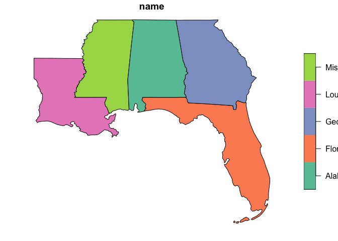
We can use the us_states() function from the USABoundaries packages
to easily define a study area based on states. This function returns a
sf object. For sf objects, there is a default plotting method that
can be used.
# Pull the boundaries for some select states for our study area
my_area <- us_states(states = c('LA','MS','AL','GA','FL'))

# Save the bounding box for later use
my_bbox <- my_area %>%
  st_bbox()

# Plot using the default plotting method for `sf` objects
plot(my_area['name'])
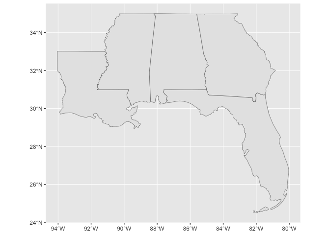
But we will use the ggplot2 functions to build more complicated maps.
With both the ggplot2 and sf packages, we can take advantage of the
geom_sf() function to quickly plot sf objects in the ggplot2
framework. Unlike most ggplot() uses, you don’t have to specify the
x and y mapping aesthetic for geom_sf() since that will be assumed
from the geometry column.
ggplot() +
  geom_sf(data=my_area)
Say you want to use a certain CRS in the project for which you are making your map. This can affect the plotted map.
# Specify the target CRS
target_crs <- 5070
target_crs_str <- paste0('EPSG:',target_crs)

# Transform area to that CRS and save the bounding box in the CRS for later use
my_area_tcrs <- my_area %>%
  st_transform(target_crs)
my_bbox_tcrs <- my_area_tcrs %>%
  st_bbox()

# Plot the transformed area
ggplot() +
  geom_sf(data=my_area_tcrs)
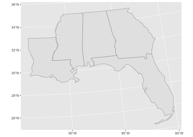
The plot coordinate system depends on the order of the geom_sf()
calls, or what’s specifically stated in coord_sf().
Let’s now consider another vector dataset we’d like to plot within our study area. We can use the GeoPlatform API to download a subset of the FS National Forests Dataset (US Forest Service Proclaimed Forests) dataset from the US Forest Service.
# GeoPlatform API url
api_url <- 'https://geoapi.geoplatform.gov'
# Read collections catalog
collections_url <- paste0(api_url,'/collections')
collections_content <- GET(collections_url) %>%
content()
collections_md <- collections_content$collections
# Get collection ID for collection with 'forest' in the title
search_term <- 'forest'
collection_titles <- sapply(collections_md, function(col) tolower(col$title))
collection_id <- collections_md[[grep(search_term,collection_titles)]]$id
# Download data within bounding box from collection
bbox_str <- paste0(my_bbox,collapse = ',')
data_url <- paste0(collections_url, "/" ,collection_id,
"/items?limit=10000&bbox=", bbox_str)
tmp_file <- 'temp.zip'
GET(data_url, write_disk(tmp_file,overwrite=TRUE))
collection_sf <- st_read(tmp_file)
# View shape
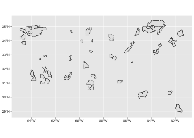
ggplot() +
geom_sf(data=collection_sf)
Now let’s plot both this forest dataset and our study area.
ggplot() +
  geom_sf(data=my_area_tcrs) +
  geom_sf(data=collection_sf)
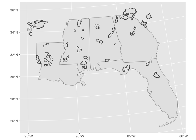
First, it is hard to distinguish the two vector datasets with the default coloring. Second, we requested forests within a bounding box of our study area. So let’s find the intersection of our forests and study area, and color the forests polygons.
my_forests_tcrs <- collection_sf %>%
  st_transform(target_crs) %>%
  st_buffer(1) %>%
  st_intersection(my_area_tcrs)

ggplot() +
  geom_sf(data=my_area_tcrs) +
  geom_sf(data=my_forests_tcrs,
          fill = 'forestgreen')
![]()
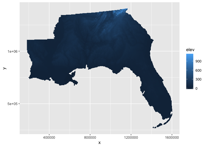
And let’s also get a raster dataset to fill in our study area. We will download some elevation from The National Map. Again, we will use our study area bounding box to define our subset.
tnm_url <- 'https://elevation.nationalmap.gov/arcgis/rest/services/'
my_raster <- 'elev.tiff'
GET(paste0(tnm_url,'3DEPElevation/ImageServer/exportImage?bbox=',bbox_str,
           '&bboxSR=4326&format=tiff&f=image'),
    write_disk(my_raster,overwrite=TRUE))

elev <- rast(my_raster)

# Visualize with default terra plotting function for rasters
plot(elev)

We will reproject this raster into our target CRS and apply a mask
defined by our study area. Then, we will also convert this terra
object into a data.frame to help with our ggplotting.
elev_masked <- elev %>%
  project(target_crs_str) %>%
  mask(my_area_tcrs)

elev_df <- elev_masked %>%
  as.data.frame(xy=TRUE)
With the default color scale, the elevation is difficult to distinguish across the study area.
elev_df %>%
  ggplot(aes(x,y,fill=elev)) +
  geom_raster()
There is an option to apply transformations within the fill color scale,
scale_fill_continuous, e.g., the square-root transform which can
increase the visual contrast in the elevation raster. However, there are
areas below sea level in our study area so these pixels will become NA
after the square-root transform.
elev_df %>%
  ggplot(aes(x,y,fill=elev)) +
  geom_raster() +
  scale_fill_continuous(trans = 'sqrt')

#> Warning in self$trans$transform(x): NaNs produced

#> Warning: Transformation introduced infinite values in discrete y-axis
![]()
You can also manually modify your raster variable being plotted to perform similar transformations, including more flexibility like an offset for our case to deal with the below sea level values. The down-side is you would also have to manually edit the legend to make it more interpretable.
elev_df %>%
  ggplot(aes(x,y,fill=sqrt(elev+50))) +
  geom_raster()
![]()
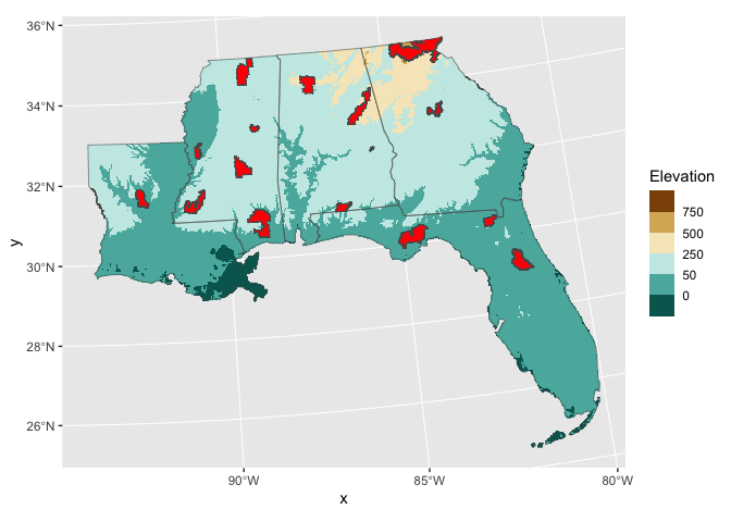
Another option is to break up your fill color scale into bins. One
option for binning continous values in ggplot2 is the
scale_*_fermenter function that relies on the RColorBrewer package.
Here, we will use this option and set manual breaks in our elevation.
ggplot() +
  geom_raster(aes(x,y,fill=elev),
              data = elev_df) +
  scale_fill_fermenter(palette = 'BrBG',
                       name = 'Elevation',
                       breaks = c(-50,0,50,250,500,750))

So here is the current state of our map with the elevation raster and the study area and forest polygons:
ggplot() +
  geom_raster(aes(x,y,fill=elev),
              data = elev_df) +
  geom_sf(data=my_area_tcrs,
          fill = NA) +
  geom_sf(data=my_forests_tcrs,
          fill = 'red') +
  scale_fill_fermenter(palette = 'BrBG',
                       name = 'Elevation',
                       breaks = c(-50,0,50,250,500,750))
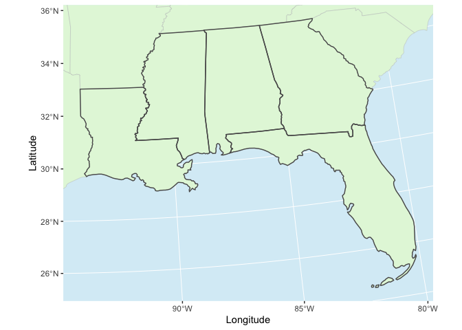
Now, we can add some nice map background layers and annotations. First,
let’s build a background to show the context of neighboring states and
water. We use the USABoundaries package again to create a US states
background and fill those states with a light green color (#e3f7dc).
We also set the panel background fill color with a light blue
(#afdbed) since this represents the water areas in the map.
all_states <- us_states() %>%
  st_transform(target_crs_str)

ggplot() +
 geom_sf(data = all_states,  #base color for all land
            fill = "#e3f7dc",
            col = "gray75",
            linewidth = 0.15) +
  geom_sf(data=my_area_tcrs,   #our study area states
          fill = NA,
          linewidth = 0.5) +
  scale_x_continuous(name = 'Longitude',   # limit axes to study area bounding box
                     limits = range(my_bbox_tcrs[c(1,3)])) +
  scale_y_continuous(name = 'Latitude',
                     limits = range(my_bbox_tcrs[c(2,4)])) +
  theme(panel.background = element_rect(fill = alpha('#afdbed', 0.5)),  # water!
        panel.grid.major = element_line(color = 'white', linewidth = 0.3))
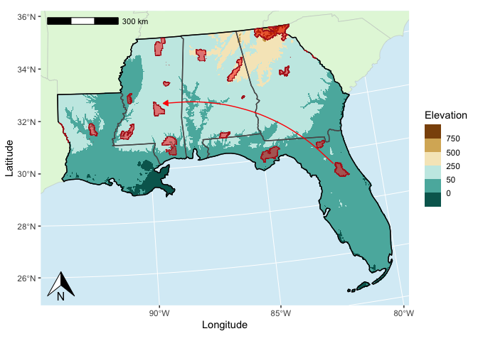
Now, let’s combine all of our incremental steps into one plot. We can also add some annotations like a north arrow, a scale bar, and some arrows.
# Define points between which to draw an arrow
arrow_pts <- data.frame(x = c(-82,-89.25),
                       y = c(29.5, 32.5)) %>%
  st_as_sf(coords = c('x','y'),
           crs = 4326) %>%
  st_transform(target_crs) %>%
  st_coordinates() %>%
  as_tibble()

# Draw the complete map
ggplot() +
 geom_sf(data = all_states,  #base color for all land
            fill = "#e3f7dc",
            col = "gray75",
            linewidth = 0.15) +
  geom_raster(aes(x,y,fill=elev),  # elevation raster
              data = elev_df) +
  geom_sf(data=my_area_tcrs,  # our study area states
          fill = NA,
          linewidth = 0.5) +
  geom_sf(data=my_area_tcrs %>%  # highlight boundary of the study area
            st_union(),
          fill = NA,
          color = 'black',
          linewidth = 0.5) +
  geom_sf(data=my_forests_tcrs, # forest polygons
          fill = 'red',
          alpha = 0.5,
          color = 'firebrick',
          linewidth = 0.25) +
  geom_curve(aes(x=arrow_pts$X[1], y = arrow_pts$Y[1],  # curved arrow
                 xend = arrow_pts$X[2], yend = arrow_pts$Y[2]),
             curvature = 0.25,
             arrow = arrow(length = unit(2,'mm'),
                           type = 'closed'),
           color = 'red') +
  scale_fill_fermenter(palette = 'BrBG',
                       name = 'Elevation',
                       breaks = c(-50,0,50,250,500,750)) +
  scale_x_continuous(name = 'Longitude',
                     limits = range(my_bbox_tcrs[c(1,3)])) +
  scale_y_continuous(name = 'Latitude',
                     limits = range(my_bbox_tcrs[c(2,4)])) +
  annotation_scale(location = "tl") +
  annotation_north_arrow(height = unit(1, "cm"),
                         width = unit(1, "cm")) +
  theme(panel.background = element_rect(fill = alpha('#afdbed', 0.5)),
        panel.grid.major = element_line(color = 'white', linewidth = 0.3))