Spatial interpolation methods: geostatistics to machine learning

Last Update: 17 September 2023
Download RMarkdown: GRWG_SpatialInterpolation.Rmd

Overview

This tutorial compares two spatial interpolation techniques that predict gridded maps of a target variable given point observations and, potentially, gridded covariates. The content of this tutorial is modified from the tutorial that is supplementary material to the scientific article: Hengl, T., Nussbaum, M., Wright, M. and Heuvelink, G.B.M., 2018. “Random Forest as a Generic Framework for Predictive Modeling of Spatial and Spatio-temporal Variables”. Modifications include limiting the number of examples and re-ordering examples, using more up-to-date R packages, and cutting and supplementing the commentary text.

To download the Rmarkdown file for this tutorial to either Ceres or Atlas within Open on Demand, you can use the following lines:

library(httr)
tutorial_name <- 'GRWG_SpatialInterpolation.Rmd'
GET(paste0('https://geospatial.101workbook.org/tutorials/',tutorial_name), 
    write_disk(tutorial_name))

Language: R

Primary Libraries/Packages:

Name	Description	Link
geoR	Analysis of Geostatistical Data	https://cran.r-project.org/web/packages/geoR/index.html
ranger	A Fast Implementation of Random Forests	https://cran.r-project.org/web/packages/ranger/index.html

Nomenclature

(Spatial) Interpolation: Using observations of dependent and independent variables to estimate the value of the dependent variable at unobserved independent variable values. For spatial applications, this can be the case of having point observations (i.e., variable observations at known x-y coordinates) and then predicting a gridded map of the variable (i.e., estimating the variable at the remaining x-y cells in the study area).
Geostatistics: Statistics focusing on spatial datasets, e.g. treating spatially heterogeneous variables as random variables with covariance structures describing spatial dependence.
Kriging: A geostatistical approach for spatial interpolatation. It uses a variogram model fitted to point observations to define spatial dependence.
Variogram: A model describing the relationship between variance between values of pairs of points as a function of the spatial distance between those points.
Random Forest: A machine learning algorithm that uses an ensemble of decision trees.

Data Details

Data: meuse data set
Link: sp package
Other Details: This dataset gives locations and topsoil heavy metal concentrations, along with a number of soil and landscape variables at the observation locations, collected in a flood plain of the river Meuse, near the village of Stein (NL). Heavy metal concentrations are from composite samples of an area of approximately 15 m x 15 m.

Analysis Steps

Pre-process the meuse data set to be sf and raster objects
Use kriging to interpolate zinc concentrations across the study area
Use Random Forest to interpolate zinc concentrations across the study area
Compare predictions and prediction error between the two interpolation methods

Step 0: Import Libraries/Packages

For this tutorial, we will use several packages for processing spatial data. The sf and raster packages help us store the meuse observations and grid in spatial data structures. geoR contains functions for fitting variograms and performing kriging. ranger contains functions to fit Random Forest models and make predictions from them.

# spatial data
library(sf)     # vector data
library(raster) # raster data

# geostatistics
library(geoR)

# random forest
library(ranger) 

# general data manipulation
library(tidyr)
library(dplyr)

# visualizations
library(ggplot2)

Step 1: Pre-process `meuse` dataset

Our dataset is contained in the sp package. We can use the demo function to load both the point observation data (new variable meuse) and the study area’s grid (new variable meuse.grid) as sp objects. Note that in most cases, defining the grid (e.g., determining the appropriate spatial resolution and extent) would be a necessary initial step based on the science question.

# This dataset is from the `sp` package, which the `raster` package
# loaded for us above.
# point observations: meuse
# study area grid: meuse.grid
demo('meuse', echo = FALSE)

We will translate these into data objects that are compatible with more recent or widely-used R packages: zinc concentration point observations into a sf object and the study area grid into a raster object.

obs_sf <- meuse['zinc'] %>%
  st_as_sf()

grid_raster <- raster(meuse.grid['soil'])

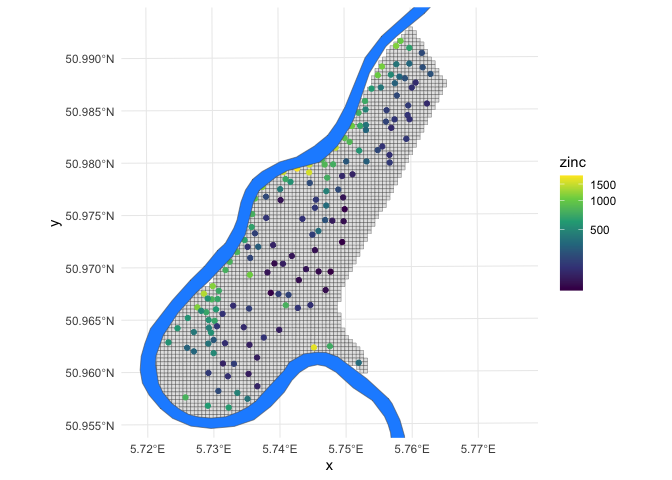
Let’s take a quick look at the dataset. Below is a map of the study area grid and the observation locations, plus the location of the river Meuse for reference (the demo call also created the meuse.riv variable, though we will only use it for visualization purposes).

grid_raster %>% 
  as.data.frame(xy = TRUE) %>%
  filter(!is.na(soil_levels)) %>% # study area only
  ggplot() +
  geom_tile(aes(x,y),
            fill = 'gray90',
            color = 'black') +
  geom_sf(data=obs_sf,
          aes(color = zinc)) +
  geom_sf(data = meuse.riv %>%
            st_as_sf(),
          fill = 'dodgerblue') +
  theme_minimal() +
  scale_y_continuous(limits = extent(grid_raster)[c(3,4)]) +
  scale_color_viridis_c(trans = 'log1p')

Step 2: Interpolate map from point observations using kriging

The first step to perform the interpolation by kriging is to fit a variogram to the point observations. Variograms are typically fit by weighted ordinary least squares with higher weights on shorter distances. Since the variogram is a non-linear function, non-linear least squares is performed. Unlike simple linear regression, initial values are required for parameters are required for non-linear least squares. So we will first plot the empirical variogram (semivariance-distance values based on observations) to inform our initial values. The geoR package has a function variog to calculate the empirical variogram and it comes with a general plotting function for plotting that empirical variogram.

variog(data = log1p(obs_sf$zinc),
       coords = obs_sf %>%
         st_coordinates()) %>% 
  plot()

#> variog: computing omnidirectional variogram

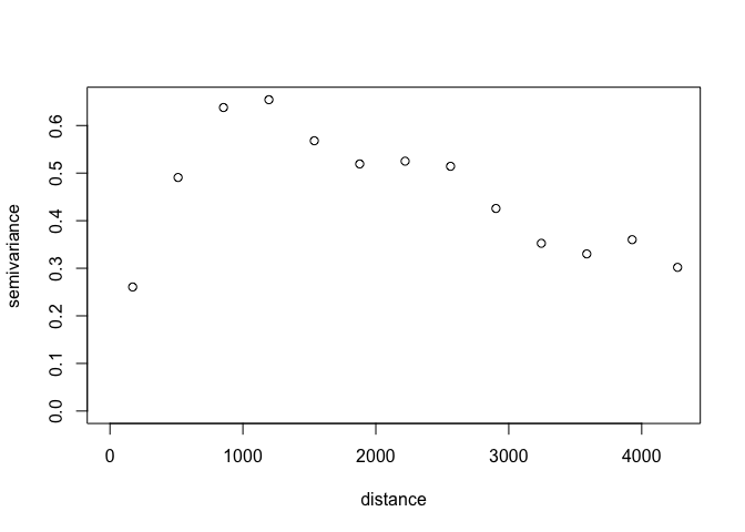
In the original tutorial, the initial value of the partial sill parameter was taken from the sample variance of all natural log-transformed zinc concentration observations and the initial values of the range parameter was 500 m. We will use these values as well.

The likfit function performs the variogram fitting based on the initial values and the empirical variogram. Zinc concentration is natural log-transformed to help meet the assumption of normality (and this is why the Box-Cox parameter lambda is set to zero).

initial_psill <- var(log1p(obs_sf$zinc))
initial_range <- 500 # meters
ini.v <- c(initial_psill,initial_range)
zinc_vgm <- likfit(data = obs_sf$zinc, 
                   coords = obs_sf %>%
                     st_coordinates(),
                   lambda=0, 
                   ini=ini.v, 
                   cov.model="exponential")

#> kappa not used for the exponential correlation function
#> ---------------------------------------------------------------
#> likfit: likelihood maximisation using the function optim.
#> likfit: Use control() to pass additional
#>          arguments for the maximisation function.
#>         For further details see documentation for optim.
#> likfit: It is highly advisable to run this function several
#>         times with different initial values for the parameters.
#> likfit: WARNING: This step can be time demanding!
#> ---------------------------------------------------------------
#> likfit: end of numerical maximisation.

zinc_vgm

#> likfit: estimated model parameters:
#>       beta      tausq    sigmasq        phi 
#> "  6.1553" "  0.0164" "  0.5928" "500.0001" 
#> Practical Range with cor=0.05 for asymptotic range: 1497.866
#> 
#> likfit: maximised log-likelihood = -1014

To generate predictions and kriging variance using geoR we run:

zinc_ok <- krige.conv(data = obs_sf$zinc, 
                      coords = obs_sf %>%
                        st_coordinates(),
                      locations=coordinates(grid_raster), 
                      krige=krige.control(obj.model=zinc_vgm)) # our fitted variogram

#> krige.conv: model with constant mean
#> krige.conv: performing the Box-Cox data transformation
#> krige.conv: back-transforming the predicted mean and variance
#> krige.conv: Kriging performed using global neighbourhood

grid_raster$zinc_ok <- zinc_ok$predict
grid_raster$zinc_ok_range <- sqrt(zinc_ok$krige.var)

grid_raster %>% 
  as.data.frame(xy = TRUE) %>%
  filter(!is.na(soil_levels)) %>% # study area only
  ggplot() +
  geom_tile(aes(x,y,fill=zinc_ok)) +
  geom_sf(data=obs_sf,
          shape = 3,
          size = 0.5) +
  scale_fill_distiller(palette = 'RdYlBu',
                       trans = 'log1p',
                       na.value = NA) +
  theme_minimal() 

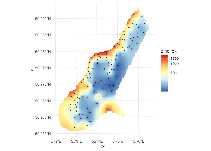
in this case geoR automatically back-transforms values to the original scale, which is a recommended feature.

Step 3: Interpolate map from point observations using Random Forest

We can derive buffer distances by generating N rasters of distances to each i=1,..,N point observations. This can be coded in multiple different ways, but the code chunk below takes the approach of using sf::st_distance() to calculate the distances.

First, we will create a list of grid cell coordinates into a sf object. Then, we iterative fill out layers in a raster brick (one layer for each observation) with the distances to each observation from every cell in the raster.

# Create a `sf` object from the raster cell center coordinates
grid_sf <- grid_raster %>%
  coordinates() %>%  # extract cell coordinates
  as_tibble() %>%  # or as.data.frame, because st_as_sf() doesn't like matrices
  st_as_sf(coords = c('x','y'),
           crs = st_crs(obs_sf)) # keep dataset's CRS


# Define an empty raster brick with N la
grid_distances <- brick(grid_raster,
                    values = FALSE,
                    nl = nrow(obs_sf))
for(i in 1:nrow(obs_sf)){
  target_pt <- obs_sf[i,]
  grid_distances[[i]] <- st_distance(grid_sf, target_pt)
}

#> Warning in readAll(x): cannot read values; there is no file associated with this RasterBrick

which takes few seconds as it generates 155 gridded maps. The value of the target variable zinc can be now modeled as a function of buffer distances:

### For each observation, what layer distance
dn0 <- paste(names(grid_distances), collapse="+")
fm0 <- as.formula(paste("zinc ~ ", dn0))
fm0

#> zinc ~ layer.1 + layer.2 + layer.3 + layer.4 + layer.5 + layer.6 + 
#>     layer.7 + layer.8 + layer.9 + layer.10 + layer.11 + layer.12 + 
#>     layer.13 + layer.14 + layer.15 + layer.16 + layer.17 + layer.18 + 
#>     layer.19 + layer.20 + layer.21 + layer.22 + layer.23 + layer.24 + 
#>     layer.25 + layer.26 + layer.27 + layer.28 + layer.29 + layer.30 + 
#>     layer.31 + layer.32 + layer.33 + layer.34 + layer.35 + layer.36 + 
#>     layer.37 + layer.38 + layer.39 + layer.40 + layer.41 + layer.42 + 
#>     layer.43 + layer.44 + layer.45 + layer.46 + layer.47 + layer.48 + 
#>     layer.49 + layer.50 + layer.51 + layer.52 + layer.53 + layer.54 + 
#>     layer.55 + layer.56 + layer.57 + layer.58 + layer.59 + layer.60 + 
#>     layer.61 + layer.62 + layer.63 + layer.64 + layer.65 + layer.66 + 
#>     layer.67 + layer.68 + layer.69 + layer.70 + layer.71 + layer.72 + 
#>     layer.73 + layer.74 + layer.75 + layer.76 + layer.77 + layer.78 + 
#>     layer.79 + layer.80 + layer.81 + layer.82 + layer.83 + layer.84 + 
#>     layer.85 + layer.86 + layer.87 + layer.88 + layer.89 + layer.90 + 
#>     layer.91 + layer.92 + layer.93 + layer.94 + layer.95 + layer.96 + 
#>     layer.97 + layer.98 + layer.99 + layer.100 + layer.101 + 
#>     layer.102 + layer.103 + layer.104 + layer.105 + layer.106 + 
#>     layer.107 + layer.108 + layer.109 + layer.110 + layer.111 + 
#>     layer.112 + layer.113 + layer.114 + layer.115 + layer.116 + 
#>     layer.117 + layer.118 + layer.119 + layer.120 + layer.121 + 
#>     layer.122 + layer.123 + layer.124 + layer.125 + layer.126 + 
#>     layer.127 + layer.128 + layer.129 + layer.130 + layer.131 + 
#>     layer.132 + layer.133 + layer.134 + layer.135 + layer.136 + 
#>     layer.137 + layer.138 + layer.139 + layer.140 + layer.141 + 
#>     layer.142 + layer.143 + layer.144 + layer.145 + layer.146 + 
#>     layer.147 + layer.148 + layer.149 + layer.150 + layer.151 + 
#>     layer.152 + layer.153 + layer.154 + layer.155

Further analysis is similar to any regression analysis using the ranger package. First we overlay points and grids to create a regression matrix:

### What are those layer values at each of the observations
obs_dist <- raster::extract(grid_distances, obs_sf)
rm_zinc <- cbind(obs_sf["zinc"], obs_dist) %>%
  as_tibble()

To also estimate the prediction error variance i.e. prediction intervals we set quantreg=TRUE which initiates the Quantile Regression RF approach:

m.zinc <- ranger(fm0, rm_zinc, quantreg=TRUE, num.trees=150, seed=1)
m.zinc

#> Ranger result
#> 
#> Call:
#>  ranger(fm0, rm_zinc, quantreg = TRUE, num.trees = 150, seed = 1) 
#> 
#> Type:                             Regression 
#> Number of trees:                  150 
#> Sample size:                      155 
#> Number of independent variables:  155 
#> Mtry:                             12 
#> Target node size:                 5 
#> Variable importance mode:         none 
#> Splitrule:                        variance 
#> OOB prediction error (MSE):       68003.69 
#> R squared (OOB):                  0.4953088

This shows that, only buffer distance explain almost 50% of variation in the target variable. To generate prediction for the zinc variable and using the RFsp model, we use:

## 1 s.d. quantiles
quantiles = c((1-.682)/2, 0.5, 1-(1-.682)/2)
zinc_rfd <- predict(m.zinc, 
                    values(grid_distances), 
                    quantiles=quantiles, 
                    type="quantiles")$predictions
str(zinc_rfd)

#>  num [1:8112, 1:3] 281 281 281 281 281 281 281 281 281 281 ...
#>  - attr(*, "dimnames")=List of 2
#>   ..$ : NULL
#>   ..$ : chr [1:3] "quantile= 0.159" "quantile= 0.5" "quantile= 0.841"

this will estimate 67% probability lower and upper limits and median value. Note that “median” can often be different from the “mean”, so if you prefer to derive mean, then the quantreg=FALSE needs to be used as the Quantile Regression Forests approach can only derive median.

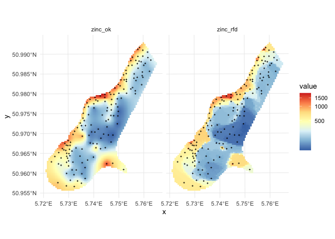
Step 4: Compare predictions and prediction error between the two interpolation methods

Comparison of predictions and prediction error maps produced using geoR (ordinary kriging) and RFsp (with buffer distances and by just using coordinates) is given below.

grid_raster$zinc_rfd = zinc_rfd[,2]
grid_raster$zinc_rfd_range = (zinc_rfd[,3]-zinc_rfd[,1])/2
grid_raster <- mask(grid_raster, grid_raster[[1]]) 

grid_raster  %>%
  as.data.frame(xy=TRUE) %>%
  dplyr::select(x,y,zinc_ok, zinc_rfd) %>%
  pivot_longer(-c(x,y)) %>%
  ggplot() +
  geom_tile(aes(x,y,fill=value)) +
  geom_sf(data=obs_sf,
          shape = 3,
          size = 0.5,
          color = 'black') +
  scale_fill_distiller(palette = 'RdYlBu',
                       trans = 'log1p',
                       na.value = NA) +
  theme_minimal() +
  facet_wrap(~name)

grid_raster  %>%
  as.data.frame(xy=TRUE) %>%
  dplyr::select(x,y,zinc_ok_range, zinc_rfd_range) %>%
  pivot_longer(-c(x,y)) %>%
  ggplot() +
  geom_tile(aes(x,y,fill=value)) +
  geom_sf(data=obs_sf,
          shape = 3,
          size = 0.5,
          color = 'black') +
  scale_fill_distiller(palette = 'RdYlBu',
                       trans = 'log1p',
                       na.value = NA) +
  theme_minimal() +
  facet_wrap(~name)

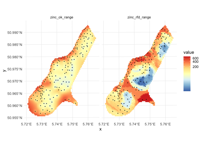
Figure: Comparison of predictions based on ordinary kriging as implemented in the geoR package (left) and random forest (right) for Zinc concentrations, Meuse data set: (first row) predicted concentrations in log-scale and (second row) standard deviation of the prediction errors for OK and RF methods.

From the plot above, it can be concluded that RFsp gives very similar results as ordinary kriging via geoR. The differences between geoR and RFsp, however, are:

RF requires no transformation i.e. works equally good with skewed and normally distributed variables; in general RF, has much less statistical assumptions than model-based geostatistics,
RF prediction error variance in average shows somewhat stronger contrast than OK variance map i.e. it emphasizes isolated less probable local points much more than geoR,
RFsp is significantly more computational as distances need to be derived from any sampling point to all new predictions locations,
geoR uses global model parameters and as such also prediction patterns are relatively uniform, RFsp on the other hand (being a tree-based) will produce patterns that as much as possible match data,

Spatial interpolation methods: geostatistics to machine learning

Heather Savoy

Overview

Nomenclature

Data Details

Analysis Steps

Step 0: Import Libraries/Packages

Step 1: Pre-process `meuse` dataset

Step 2: Interpolate map from point observations using kriging

Step 3: Interpolate map from point observations using Random Forest

Step 4: Compare predictions and prediction error between the two interpolation methods

Further reading / more complicated examples

Spatial interpolation methods: geostatistics to machine learning

Heather Savoy

Overview

Nomenclature

Data Details

Analysis Steps

Step 0: Import Libraries/Packages

Step 1: Pre-process meuse dataset

Step 2: Interpolate map from point observations using kriging

Step 3: Interpolate map from point observations using Random Forest

Step 4: Compare predictions and prediction error between the two interpolation methods

Further reading / more complicated examples

Step 1: Pre-process `meuse` dataset