
Last Update: 4 January 2024
Download Jupyter Notebook: GRWG23_SpatialInterpolation_python.ipynb
Overview
This tutorial will implement and compare machine learning techniques with two approaches to including spatial proximity for spatial modeling tasks:
- Spatial interpolation from point observations
- Spatial prediction from point observations and gridded covariates
Language: Python
Primary Libraries/Packages:
| Name | Description | Link |
|---|---|---|
pandas |
Dataframes and other datatypes for data analysis and manipulation | https://pandas.pydata.org/ |
geopandas |
Extends datatypes used by pandas to allow spatial operations on geometric types | https://geopandas.org/en/stable/ |
scikit-learn |
Machine Learning in Python | https://scikit-learn.org/stable/ |
plotnine |
A plotting library for Python modeled after R’s ggplot2 | https://plotnine.readthedocs.io/en/v0.12.3/ |
Nomenclature
- (Spatial) Interpolation: Using observations of dependent and independent variables to estimate the value of the dependent variable at unobserved independent variable values. For spatial applications, this can be the case of having point observations (i.e., variable observations at known x-y coordinates) and then predicting a gridded map of the variable (i.e., estimating the variable at the remaining x-y cells in the study area).
- Random Forest: A supervised machine learning algorithm that uses an ensemble of decision trees for regression or classification.
Tutorial Steps
- 1. Read in and visualize point observations
- 2. Random Forest for spatial interpolation
Use Random Forest to interpolate zinc concentrations across the study area in two ways:
- 2.a. RFsp: distance to all observations
- 2.b. RFSI: n observed values and distance to those n observation locations
- 3. Bringing in gridded covariates
Step 0: Load libraries and define function
First, we will import required packages and set a large default figure size. We will also define a function to print model metrics.
from sklearn.ensemble import RandomForestRegressor
from sklearn.metrics import r2_score, mean_squared_error
from sklearn.model_selection import train_test_split, RandomizedSearchCV
from scipy.stats import randint
import geopandas as gpd
import pandas as pd
import numpy as np
import plotnine as pn

pn.options.figure_size = (10, 10)
def print_metrics(y_test, y_pred):
    """
    Given observed and predicted y values, print the R^2 and RMSE metrics.

    y_test (Series): The observed y values.
    y_pred (Series): The predicted y values.
    """
    # R^2
    r2 = r2_score(y_test, y_pred)
    # Root mean squared error - RMSE
    rmse = mean_squared_error(y_test, y_pred, squared = False)
    print("R^2 = {0:3.2f}, RMSE = {1:5.0f}".format(r2,rmse))
Step 1: Read in and visualize point observations
We will open three vector datasets representing the point observations, the grid across which we want to predict, and the location of the river surrounding the study area.
This dataset gives locations and topsoil heavy metal concentrations, along with a number of soil and landscape variables at the observation locations, collected in a flood plain of the river Meuse, near the village of Stein (NL). Heavy metal concentrations are from composite samples of an area of approximately 15 m x 15 m. The data were extracted from the sp R package.
dnld_url = 'https://geospatial.101workbook.org/SpatialModeling/assets/'
# Point observations and study area grid
meuse_obs = gpd.read_file(dnld_url + 'meuse_obs.zip')
meuse_grid = gpd.read_file(dnld_url + 'meuse_grid.zip')

# Extra information for visualization:
xmin, ymin, xmax, ymax = meuse_grid.total_bounds
meuse_riv = gpd.read_file(dnld_url + 'meuse_riv.zip')
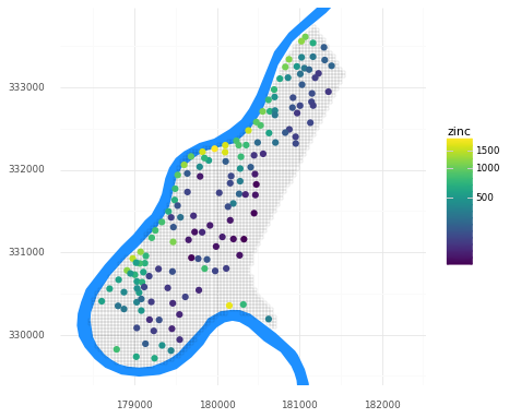
Let’s take a quick look at the dataset. Below is a map of the study area grid and the observation locations, plus the location of the river Meuse for reference. We can see that observed zinc concentrations tend to be higher closer to the river.
(pn.ggplot()
    + pn.geom_map(meuse_riv, fill = '#1e90ff', color = None)
    + pn.geom_map(meuse_grid, fill = None, size = 0.05)
    + pn.geom_map(meuse_obs, pn.aes(fill = 'zinc'), color = None, size = 3)
    + pn.scale_y_continuous(limits = [ymin, ymax])
    + pn.scale_fill_continuous(trans = 'log1p')
    + pn.theme_minimal()
    + pn.coord_fixed()
)
Step 2: Random Forest for spatial interpolation
We will explore two methods from recent literature that combine spatial proximity information as variables in fitting Random Forest models for spatial interpolation.
Step 2a: RFsp: distance to all observations
First, we will implement the RFsp method from Hengl et al 2018. This method involves using the distance to every observation as a predictor. For example, if there are 10 observations of the target variable, then there would be 10 predictor variables with the ith predictor variable representing the distance to the ith observation.
If you want to learn more about this approach, see the thengl/GeoMLA GitHub repo or the Spatial and spatiotemporal interpolation using Ensemble Machine Learning site from the same creators. Note: these resources are for R, but the latter does mention the scikit-learn library in Python that we will be using in this tutorial.
To start, we will generate two DataFrames of distances:
- One with rows representing observations and columns representing observations (these will be our data for fitting and testing the model)
- One with rows representing grid cell centers and columns representing observations (these will be how we estimate maps of our target variable with the final model)
# Get coordinates of grid cell centers - these are our locations at which we will
# want to interpolate our target variable.
grid_centers = meuse_grid.centroid

# Generate a grid of distances to each observation
grid_distances = pd.DataFrame()
# We also need the distance values among our observations
obs_distances = pd.DataFrame()

# We need a dataframe with rows representing prediction grid cells
# (or observations)
# and columns representing observations
for obs_index in range(meuse_obs.geometry.size):
    cur_obs = meuse_obs.geometry.iloc[obs_index]
    obs_name = 'obs_' + str(obs_index)

    cell_to_obs = grid_centers.distance(cur_obs).rename(obs_name)
    grid_distances = pd.concat([grid_distances, cell_to_obs], axis=1)

    obs_to_obs = meuse_obs.distance(cur_obs).rename(obs_name)
    obs_distances = pd.concat([obs_distances, obs_to_obs], axis=1)
Before moving on to model fitting, let’s take a look at the distance matrices we created.
obs_distances
| obs_0 | obs_1 | obs_2 | obs_3 | obs_4 | obs_5 | obs_6 | obs_7 | obs_8 | obs_9 | ... | obs_145 | obs_146 | obs_147 | obs_148 | obs_149 | obs_150 | obs_151 | obs_152 | obs_153 | obs_154 | |
|---|---|---|---|---|---|---|---|---|---|---|---|---|---|---|---|---|---|---|---|---|---|
| 0 | 0.000000 | 70.837843 | 118.848643 | 259.239272 | 366.314073 | 473.629602 | 258.321505 | 252.049598 | 380.189426 | 471.008492 | ... | 4304.014173 | 4385.565870 | 4425.191182 | 4194.974374 | 4077.205538 | 3914.407363 | 3868.323926 | 3964.443088 | 3607.233843 | 3449.821155 |
| 1 | 70.837843 | 0.000000 | 141.566239 | 282.851551 | 362.640318 | 471.199533 | 234.401365 | 195.010256 | 328.867755 | 441.530293 | ... | 4236.122756 | 4316.784220 | 4355.550137 | 4126.296645 | 4007.817486 | 3845.342247 | 3798.730841 | 3894.291848 | 3538.899546 | 3391.434505 |
| 2 | 118.848643 | 141.566239 | 0.000000 | 143.171226 | 251.023903 | 356.866922 | 167.000000 | 222.081066 | 323.513524 | 375.033332 | ... | 4278.052010 | 4365.122793 | 4411.447155 | 4173.908121 | 4061.434476 | 3896.201483 | 3854.403326 | 3956.156721 | 3584.262407 | 3389.963569 |
| 3 | 259.239272 | 282.851551 | 143.171226 | 0.000000 | 154.262763 | 242.156974 | 175.171345 | 296.786118 | 347.351407 | 322.818835 | ... | 4292.750750 | 4386.465206 | 4440.764349 | 4194.687712 | 4088.695146 | 3920.739726 | 3884.100024 | 3992.349935 | 3603.447377 | 3361.647959 |
| 4 | 366.314073 | 362.640318 | 251.023903 | 154.262763 | 0.000000 | 108.577162 | 147.526269 | 281.937936 | 266.101484 | 178.518907 | ... | 4162.607356 | 4260.340127 | 4319.896411 | 4068.314639 | 3966.640014 | 3796.976824 | 3763.871411 | 3876.723488 | 3476.475514 | 3212.786952 |
| ... | ... | ... | ... | ... | ... | ... | ... | ... | ... | ... | ... | ... | ... | ... | ... | ... | ... | ... | ... | ... | ... |
| 150 | 3914.407363 | 3845.342247 | 3896.201483 | 3920.739726 | 3796.976824 | 3786.887904 | 3753.359162 | 3676.331051 | 3579.912988 | 3620.842443 | ... | 471.958685 | 476.656060 | 536.660041 | 296.082759 | 183.619171 | 0.000000 | 147.989865 | 334.846233 | 345.144897 | 1443.022176 |
| 151 | 3868.323926 | 3798.730841 | 3854.403326 | 3884.100024 | 3763.871411 | 3757.931479 | 3714.900268 | 3633.511387 | 3540.952697 | 3589.008916 | ... | 599.736609 | 562.318415 | 557.046677 | 405.097519 | 217.082933 | 147.989865 | 0.000000 | 210.857772 | 391.256949 | 1545.369859 |
| 152 | 3964.443088 | 3894.291848 | 3956.156721 | 3992.349935 | 3876.723488 | 3875.800046 | 3821.201513 | 3734.408655 | 3647.002194 | 3703.768081 | ... | 702.359595 | 596.896138 | 497.033198 | 494.814107 | 276.524863 | 334.846233 | 210.857772 | 0.000000 | 595.131078 | 1756.173397 |
| 153 | 3607.233843 | 3538.899546 | 3584.262407 | 3603.447377 | 3476.475514 | 3462.718152 | 3438.127688 | 3365.864673 | 3265.476382 | 3299.412827 | ... | 702.659235 | 784.390209 | 880.273253 | 592.150319 | 528.674758 | 345.144897 | 391.256949 | 595.131078 | 0.000000 | 1176.606136 |
| 154 | 3449.821155 | 3391.434505 | 3389.963569 | 3361.647959 | 3212.786952 | 3163.395170 | 3225.188987 | 3198.113350 | 3071.672183 | 3038.833493 | ... | 1461.677119 | 1666.870721 | 1877.419772 | 1521.862017 | 1600.647681 | 1443.022176 | 1545.369859 | 1756.173397 | 1176.606136 | 0.000000 |
155 rows × 155 columns
For fitting our model, we will use the distances among observations as our predictors and observed zinc concentration at those observations as our target variable.
# matrix of distance to observations as predictors
RFsp_X = obs_distances
# vector of observed zinc concentration as target variable
y = meuse_obs['zinc']

# We need to split our dataset into train and test datasets. We'll use 80% of
# the data for model training.
RFsp_X_train, RFsp_X_test, RFsp_y_train, RFsp_y_test = train_test_split(RFsp_X, y, train_size=0.8)
Machine learning algorithms typically have hyperparameters that can be tuned per application. Here, we will tune the number of trees in the random forest model and the maximum depth of the trees in the the random forest model. We use the training subset of our data for this fitting and tuning process. After the code chunk below, the best parameter values from our search are printed.
r_state = 0

# Define the parameter space that will be searched over.
param_distributions = {'n_estimators': randint(1, 100),
                       'max_depth': randint(5, 10)}

# Now create a searchCV object and fit it to the data.
tuned_RFsp = RandomizedSearchCV(estimator=RandomForestRegressor(random_state=r_state),
                            n_iter=10,
                            param_distributions=param_distributions,
                            random_state=r_state).fit(RFsp_X_train, RFsp_y_train)
tuned_RFsp.best_params_
{'max_depth': 7, 'n_estimators': 37}
We can now use our testing subset of the data to quantify the model performance, i.e. how well did the model predict the remaining observed values? There are many potential metrics - see all the metrics scikit-learn supports here. The two we show below are the coefficient of determination (R2) and the root mean square error (RMSE), two metrics that are likely familiar from outside machine learning as well.
print_metrics(RFsp_y_test, tuned_RFsp.predict(RFsp_X_test))
R^2 = 0.50, RMSE = 286
Our R2 is not awesome! We typically want R2 values closer to 1 and RMSE values closer to 0. Note: RMSE is in the units of the target variable, so our zinc concentrations. You can see the range of values of zinc concentrations in the legend in the figure above, from which you can get a sense of our error.
Excercise: Modify the param_distributions and n_iter values above - can you improve the metrics? Note that you may also increase the processing time.
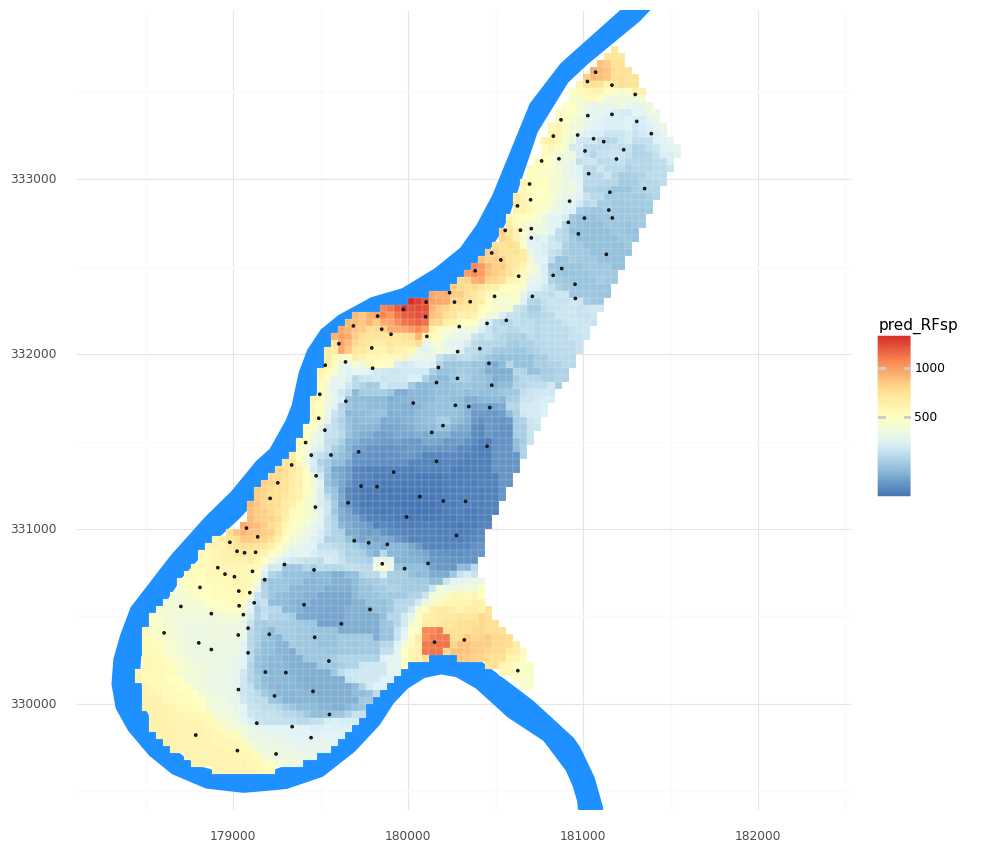
Once we are happy with (or at least curious about!) the model, we can predict and visualize our zinc concentration field.
# Predict the value from all grid cells using their distances we determined above.
meuse_grid['pred_RFsp'] = tuned_RFsp.predict(grid_distances)

(pn.ggplot()
    + pn.geom_map(meuse_riv, fill = '#1e90ff', color = None)
    + pn.geom_map(meuse_grid, pn.aes(fill = 'pred_RFsp'), color = 'white', size = 0.05)
    + pn.geom_map(meuse_obs)
    + pn.scale_y_continuous(limits = [ymin, ymax])
    + pn.scale_fill_distiller(type = 'div', palette = 'RdYlBu',trans = 'log1p')
    + pn.theme_minimal()
    + pn.coord_fixed()
)
2b: RFSI: n observed values and distance to those n observation locations
Now, we will try the the RFSI method from Sekulić et al 2020. In this method, instead of using distances to all observations as our predictors, we will use distances to the n closest observations as well as the observed values at those locations as our predictors.
Below, we define a function to find the n closest observations and record their distances and values.
def nclosest_dist_value(dist_ij, obs_i, n = 3):
    """
    Given a distance matrix among i locations and j observation
    locations, j observed values, and the number of close
    observations desired, generates a dataframe of distances to
    and values at n closest observations for each of the i
    locations.

    dist_ij (DataFrame): distance matrix among i locations and j
    observation locations
    obs_i (Series): The i observed values
    n (int): The desired number of closest observations
    """
    # Which observations are the n closest?
    # But do not include distance to oneself.
    # Note: ranks start at 1, not 0.
    nclosest_dist_ij =  dist_ij.replace(0.0,np.nan).rank(axis = 1, method = 'first') <= n

    nclosest = pd.DataFrame()

    # For each observation, find the n nearest observations and
    # record the distance and target variable pairs
    for i in range(dist_ij.shape[0]):
        # Which obs are the n closest to the ith location?
        nclosest_j_indices = np.where(nclosest_dist_ij.iloc[i,:])

        # Save the distance to and observed value at the n closest
        # observations from the ith location
        i_loc_dist = dist_ij.iloc[i].iloc[nclosest_j_indices]
        sort_indices = i_loc_dist.values.argsort()
        i_loc_dist = i_loc_dist.iloc[sort_indices]
        i_loc_dist.rename(lambda x: 'dist' + str(np.where(x == i_loc_dist.index)[0][0]), inplace=True)

        i_loc_value = obs_i.iloc[nclosest_j_indices]
        i_loc_value = i_loc_value.iloc[sort_indices]
        i_loc_value.rename(lambda x: 'obs' + str(np.where(x == i_loc_value.index)[0][0]), inplace=True)
        i_loc = pd.concat([i_loc_dist,i_loc_value],axis = 0)
        nclosest = pd.concat([nclosest, pd.DataFrame(i_loc).transpose()], axis = 0)

    return nclosest
Let’s now use that function to find and describe the n closest observations to each obsersevation and each grid cell. Note that we are taking advantage of the obs_distances and grid_distances variables we created for the RFsp approach.
n = 10
obs_nclosest_obs = nclosest_dist_value(obs_distances, meuse_obs['zinc'], n)
grid_nclosest_obs = nclosest_dist_value(grid_distances, meuse_obs['zinc'], n)
Let’s take a closer look at our new distance matrices.
obs_nclosest_obs
| dist0 | dist1 | dist2 | dist3 | dist4 | dist5 | dist6 | dist7 | dist8 | dist9 | obs0 | obs1 | obs2 | obs3 | obs4 | obs5 | obs6 | obs7 | obs8 | obs9 | |
|---|---|---|---|---|---|---|---|---|---|---|---|---|---|---|---|---|---|---|---|---|
| 0 | 70.837843 | 118.848643 | 252.049598 | 258.321505 | 259.239272 | 336.434243 | 366.314073 | 373.483601 | 380.189426 | 399.656102 | 1141.0 | 640.0 | 406.0 | 346.0 | 257.0 | 1096.0 | 269.0 | 504.0 | 347.0 | 279.0 |
| 0 | 70.837843 | 141.566239 | 195.010256 | 234.401365 | 266.011278 | 282.851551 | 311.081983 | 328.867755 | 356.349547 | 362.640318 | 1022.0 | 640.0 | 406.0 | 346.0 | 1096.0 | 257.0 | 504.0 | 347.0 | 279.0 | 269.0 |
| 0 | 118.848643 | 141.566239 | 143.171226 | 167.000000 | 222.081066 | 251.023903 | 323.513524 | 326.401593 | 345.891602 | 351.973010 | 1022.0 | 1141.0 | 257.0 | 346.0 | 406.0 | 269.0 | 347.0 | 279.0 | 504.0 | 1096.0 |
| 0 | 143.171226 | 154.262763 | 175.171345 | 242.156974 | 259.239272 | 282.851551 | 296.786118 | 322.818835 | 324.499615 | 347.351407 | 640.0 | 269.0 | 346.0 | 281.0 | 1022.0 | 1141.0 | 406.0 | 183.0 | 279.0 | 347.0 |
| 0 | 108.577162 | 147.526269 | 154.262763 | 178.518907 | 221.758878 | 244.296950 | 251.023903 | 266.101484 | 281.937936 | 340.847473 | 281.0 | 346.0 | 257.0 | 183.0 | 279.0 | 189.0 | 640.0 | 347.0 | 406.0 | 326.0 |
| ... | ... | ... | ... | ... | ... | ... | ... | ... | ... | ... | ... | ... | ... | ... | ... | ... | ... | ... | ... | ... |
| 0 | 117.038455 | 145.602198 | 147.989865 | 183.619171 | 217.117480 | 262.619497 | 269.818457 | 293.400750 | 296.082759 | 334.846233 | 224.0 | 189.0 | 496.0 | 214.0 | 187.0 | 400.0 | 296.0 | 154.0 | 258.0 | 342.0 |
| 0 | 116.361506 | 141.000000 | 147.989865 | 160.863296 | 210.857772 | 217.082933 | 219.665655 | 243.772435 | 273.791892 | 287.702972 | 400.0 | 296.0 | 166.0 | 187.0 | 342.0 | 214.0 | 539.0 | 224.0 | 451.0 | 332.0 |
| 0 | 81.412530 | 174.942848 | 205.000000 | 210.857772 | 242.866218 | 270.351623 | 276.524863 | 286.225436 | 296.278585 | 301.317109 | 332.0 | 400.0 | 420.0 | 496.0 | 296.0 | 539.0 | 214.0 | 553.0 | 451.0 | 577.0 |
| 0 | 158.294030 | 170.390727 | 195.747286 | 260.555176 | 260.823695 | 309.161770 | 345.144897 | 353.747085 | 384.532183 | 385.020779 | 155.0 | 199.0 | 180.0 | 187.0 | 224.0 | 154.0 | 166.0 | 157.0 | 296.0 | 226.0 |
| 0 | 353.004249 | 503.135171 | 799.335974 | 848.958185 | 870.917907 | 914.617406 | 986.887025 | 1013.126349 | 1038.171469 | 1043.985153 | 722.0 | 1672.0 | 192.0 | 130.0 | 203.0 | 157.0 | 778.0 | 113.0 | 240.0 | 199.0 |
155 rows × 20 columns
We will then use the same model fitting process as for RFsp.
# matrix of distances to and observed values at the n closest observations as predictors
RFSI_X = obs_nclosest_obs

# We need to split our dataset into train and test datasets. We'll use 80% of
# the data for model training.
RFSI_X_train, RFSI_X_test, RFSI_y_train, RFSI_y_test = train_test_split(RFSI_X, y, train_size=0.8)

param_distributions = {'n_estimators': randint(1, 100),
                       'max_depth': randint(5, 10)}
tuned_RFSI  = RandomizedSearchCV(estimator=RandomForestRegressor(random_state=r_state),
                            n_iter=10,
                            param_distributions=param_distributions,
                            random_state=r_state).fit(RFSI_X_train, RFSI_y_train)
tuned_RFSI.best_params_
{'max_depth': 9, 'n_estimators': 59}
print_metrics(RFSI_y_test, tuned_RFSI.predict(RFSI_X_test))
R^2 = 0.45, RMSE = 302
How does RFSI’s metrics compare to RFsp’s? What if you modify n, the number of closest observations? What if you modify the param_distributions and n_iter values like above?
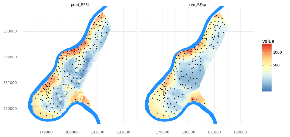
Let’s visualize the two maps from these two methods together. To do so, we will need to transform our meuse_grid DataFrame into a longer format for plotting with facets in plotnine.
meuse_grid['pred_RFSI'] = tuned_RFSI.predict(grid_nclosest_obs)
meuse_grid_long = pd.melt(meuse_grid, id_vars= 'geometry', value_vars=['pred_RFsp','pred_RFSI'])

(pn.ggplot()
    + pn.geom_map(meuse_riv, fill = '#1e90ff', color = None)
    + pn.geom_map(meuse_grid_long, pn.aes(fill = 'value'), color = 'white', size = 0.05)
    + pn.geom_map(meuse_obs)
    + pn.scale_y_continuous(limits = [ymin, ymax])
    + pn.scale_fill_distiller(type = 'div', palette = 'RdYlBu',trans = 'log1p')
    + pn.theme_minimal()
    + pn.coord_fixed()
    + pn.facet_wrap('variable')
)
Step 3: Bringing in gridded covariates
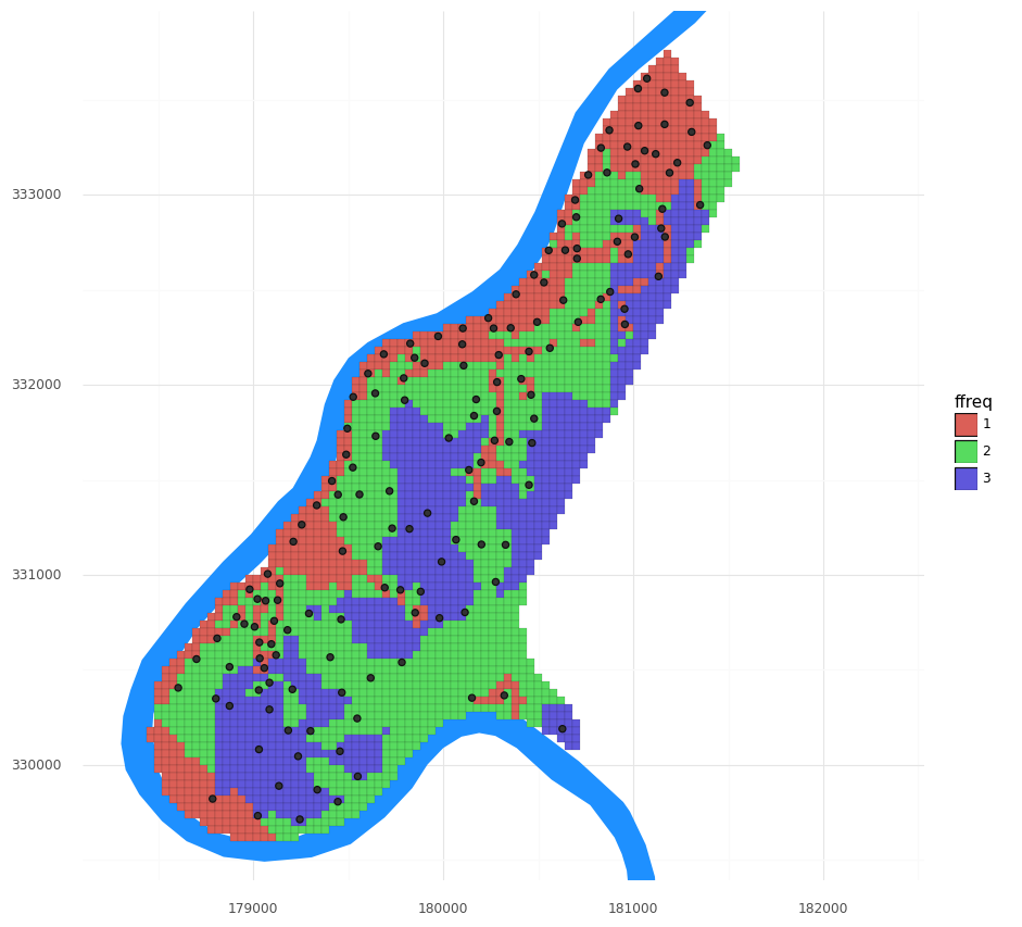
This dataset has three covariates supplied with the grid and the observations:
- dist: the distance to the river
- ffreq: a category describing the flooding frequency
- soil: a category of soil type
We can extend this spatial interpolation task into a more general spatial prediction task by including these co-located observations and gridded covariates. Let’s visualize the flooding frequency:
(pn.ggplot()
    + pn.geom_map(meuse_riv, fill = '#1e90ff', color = None)
    + pn.geom_map(meuse_grid, pn.aes(fill = 'ffreq'), size = 0.05)
    + pn.geom_map(meuse_obs, size = 2)
    + pn.scale_y_continuous(limits = [ymin, ymax])
    + pn.theme_minimal()
    + pn.coord_fixed()
)
Also visualize the other covariates. (Either one at a time, or try melting like above to use facets!). Do you expect these variables to improve the model?
Adding these covariates to the RF model, either method, is straightforward. We will stick to just the RFSI model here. All that needs to be done is to concatenate these three columns to our distance (and observed values) dataset and repeat the modeling fitting process.
# matrix of distances to and observed values at the n closest observations as predictors
RFSI_wcov_X = pd.concat([obs_nclosest_obs.reset_index(),meuse_obs[['dist','ffreq','soil']]], axis=1)

# We need to split our dataset into train and test datasets. We'll use 80% of
# the data for model training.
RFSI_wcov_X_train, RFSI_wcov_X_test, RFSI_wcov_y_train, RFSI_wcov_y_test = train_test_split(RFSI_wcov_X, y, train_size=0.8)

param_distributions = {'n_estimators': randint(1, 100),
                       'max_depth': randint(5, 10)}
tuned_RFSI_wcov = RandomizedSearchCV(estimator=RandomForestRegressor(random_state=r_state),
                            n_iter=10,
                            param_distributions=param_distributions,
                            random_state=r_state).fit(RFSI_wcov_X_train, RFSI_wcov_y_train)
tuned_RFSI_wcov.best_params_
{'max_depth': 5, 'n_estimators': 68}
print_metrics(RFSI_wcov_y_test, tuned_RFSI_wcov.predict(RFSI_wcov_X_test))
R^2 = 0.56, RMSE = 260
How did the new covariates change our metrics? Was it as you’d expect?
grid_nclosest_obs_wcov = pd.concat([grid_nclosest_obs.reset_index(),meuse_grid[['dist','ffreq','soil']]], axis=1)
meuse_grid['pred_RFSI_wcov'] = tuned_RFSI_wcov.predict(grid_nclosest_obs_wcov)
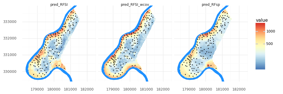
meuse_grid_long = pd.melt(meuse_grid, id_vars= 'geometry', value_vars=['pred_RFsp','pred_RFSI','pred_RFSI_wcov'])
(pn.ggplot()
+ pn.geom_map(meuse_riv, fill = '#1e90ff', color = None)
+ pn.geom_map(meuse_grid_long, pn.aes(fill = 'value'), color = 'white', size = 0.05)
+ pn.geom_map(meuse_obs, size = 0.25)
+ pn.scale_y_continuous(limits = [ymin, ymax])
+ pn.scale_fill_distiller(type = 'div', palette = 'RdYlBu',trans = 'log1p')
+ pn.theme_minimal()
+ pn.coord_fixed()
+ pn.facet_wrap('variable')
)
Use the covariates to create a RFsp_wcov model and add it to the figure. How do the metrics compare to the other results?